
Breast cancer accounts for 30% of new cancer in women in the United States, according to the American Cancer Society1. Survival analysis is used to evaluate the effectiveness of different treatments, identify factors that influence survival, and understand the probability of survival over time. I set out to train a number of machine learning models to predict probability of survival, compare them against a baseline, and identify which provides the best prediction accuracy. We were also curious to discover which clinical and genetic features are most impactful in predicting overall survival.
Thanks to my collaborator on this project, Okyaz Eminaga, who was a pleasure to work with and provided patient guidance and feedback. All mistakes and transgressions are mine alone.
All the code, including training and running the models is available here.
Data Set
The raw dataset was sourced from The Cancer Genome Atlas (TCGA) Breast Cancer (BRCA) cohort of 1,236 patients hosted by Xena2 here. I combined the following into one tabular dataset, joining on sample ID:
- RNASeq gene expression (20,531 genes X 1,218 samples)
- Clinical data (1,247 samples X 194 clinical attributes)
- Curated Survival data (1,236 samples X 11 survival attributes)
This dataset follows patient events in the cohort for twenty-three years.
Prediction Target
The prediction target is overall survival, which consists of a boolean and an event time in days. A True value for the boolean indicates loss of life caused by the disease. A False value indicates a “censor3” event, which means the patient dropped out of the cohort for another reason. Here’s a sample of what this data looks like.

In order to compare model predictive performance at various time horizons over the 23 year duration of the study, we created one, three, five and seven year targets in addition to the end of study target.
The scikit-survival candidate models we tested, Cox Proportional Hazards (“Cox PH”) and Gradient Boosting, are specifically designed for this sort of data and predict survival probability over time for the target time period.
For the other “vanilla” models we tested, Logistic Regression and XG Boost, I framed the problem as binary classification. These models predict overall survival at the end of the target time period.
All of these models can be compared apples-to-apples using the C-Index metric for survival model accuracy.
Exploratory Data Analysis
I created a number of visualizations to help me understand the datasets and quality issues that needed to be addressed, starting with a heatmap of gene expression by sample.

What if we sort genes by mean expression percentage?

The Kaplan-Meier Survival Function charts the probability of survival of patients in the cohort over the 23 year life of the study.
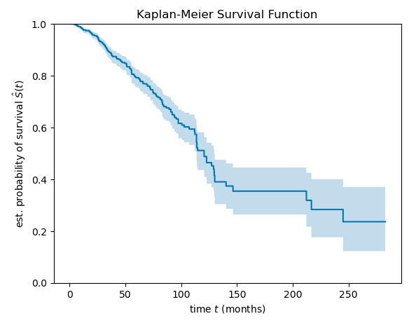
The curve starts out at probability of 1.0 that all patients are alive at the start of the study. The probability declines steadily over the first approximately eight years of the study when the bulk of the data is collected. The curve becomes more jagged and sparse as the frequency of data points collected decreases.
Here’s how the survival curve breaks down by surgical procedure…
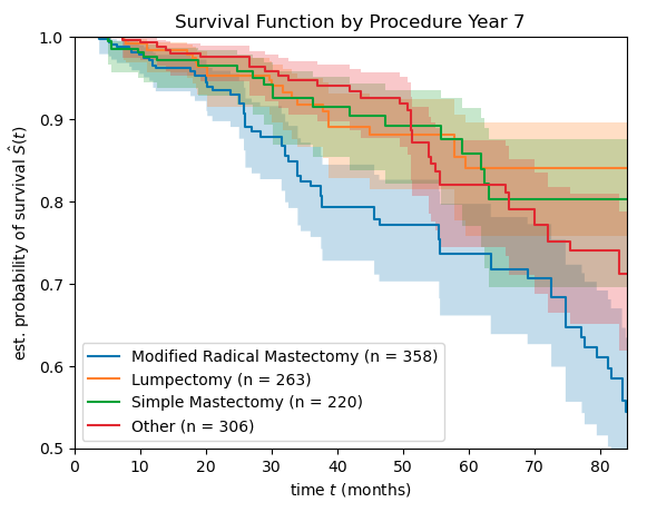
At the seven year mark in this study, patients undergoing lumpectomy or simple mastectomy seem to have a better prognosis compared to patients undergoing radical mastectomy and “Other” surgical procedure.
Data Clean Up
The data set had a number of problems and issues that were cleaned up.
- Removed genes with value of zero for all samples
- Removed one sample that had no data for PFI.time, DSS.time and OS.time
- Imputed year_of_initial_pathologic_diagnosis for 2 samples where it was missing. Replaced the two missing values with the mean.
- There were a number of features causing leakage, so removed them: days_to_death, Days_to_date_of_Death_nature2012, days_to_last_followup, days_to_last_known_alive, DSS, DFI, PFI
- Many of the clinical features were very sparse, and we removed all that contained missing values
Other Data Pre-Processing and Preparation
We used the scikit-learn StandardScaler to scale the data and promote convergence of the models.
The dataset was split 80/20 between training set and test set for final evaluation and results.
Feature Engineering
Feature engineering was not a major focus of this modeling effort. There was more emphasis on feature selection.
Steps were added to the scikit-learn pipeline for one-hot encoding a number of nominal categorical features:
- ER_Status_nature2012
- HER2_Final_Status_nature2012
- Metastasis_nature2012
- Node_nature2012
- Tumor_nature2012
The pipeline includes a step for encoding of one ordinal categorical feature, AJCC_Stage_nature20124.
Feature Selection
With 20,000+ genes in the dataset for each sample, we used an approach inspired by this paper5 to filter down to the ~900 highest information and most predictive genes…
- Filter out highly correlated genes, where correlation > 0.856
- This knocked out ~842 genes
- Filter out genes with low variation in expression %, where standard deviation < 17%
- This knocked out ~18,750 genes
This leaves us with around 927 genes in our feature dataset.
The next step in the pipeline is using SelectKBest to select the top 25 features by feature importance.
The final step in feature selection is model specific recursive feature elimination with cross validation.
Here’s the final feature list for each model…
| Cox Proportional Hazards | Gradient Boosting | Logistic Regression |
| age_at_initial_pathologic_diagnosis | age_at_initial_pathologic_diagnosis | age_at_initial_pathologic_diagnosis |
| FSIP1 | CLIC6 | HSPA2 |
| L1CAM | MAPT | AJCC_Stage_nature2012 |
| HSPA2 | HSPA2 | PDZD2 |
| PDZD2 | AJCC_Stage_nature2012 | L1CAM |
| RASGRP1 | FAM176B | |
| HPN | ||
| ELOVL2 | ||
| AJCC_Stage_nature2012 |
Build and Train Candidate Models
Scikit-learn pipelines were built for feature selection, model training and accuracy evaluation of a number of candidate algorithms at each of a number of target time horizons. Firstly, these candidate algorithms from the scikit-survival library that are specifically designed for survival analysis…
- Cox Proportional Hazards (CoxPH)
- Gradient Boosting Survival Analysis (GBSA)
Also for comparison, we tested these “vanilla” algorithms…
- XGBoost (XGB)
- Logistic Regression (Log Reg)
All the code, including training and running the models is available here.
Model Evaluation and Results
Concordance Index (C-Index) is a generally accepted evaluation metric for survival models, and that’s what we used to evaluate our models. A C-Index of 0.5 means the model provides the same accuracy as coin-flip chance. A C-Index value of 1.0 means perfect prediction accuracy for overall survival.
There are a number of sources7 suggesting that a C-Index score of 0.7 is “good” for this type of study, so that’s where we set the benchmark for accuracy of the models we built.
Here are the prediction accuracy results for the models measured as C-Index when applied to the test set.

| Model | Year 1 | Year 3 | Year 5 | Year 7 | Year 23 End of Study |
| Scikit-survival Cox PH | 0.68 | 0.73 | 0.63 | 0.70 | 0.43 |
| Scikit-survival Gradient Boosting | 0.64 | 0.72 | 0.68 | 0.63 | 0.38 |
| Logistic Regression | 0.71 | 0.70 | 0.62 | 0.59 | 0.53 |
| XG Boost | 0.56 | 0.63 | 0.64 | 0.56 | 0.58 |
There were three algorithms that beat the 0.7 “good” C-Index benchmark
- Scikit-survival Cox PH with the 3 year horizon dataset, C-Index=0.734
- Scikit-survival Gradient Boosting with the 3 year horizon dataset, C-Index=0.721
- Scikit-learn Logistic Regression with the 1 year horizon dataset, C-Index=0.713
Cox PH and Gradient Boosting have a significant increase in prediction accuracy from Year 1 to Year 3, followed by a plateau through Year 7, and a correlated drop-off to Year 23, the last event in the dataset.
The scikit-survival models predict survival over time. This chart shows how each of those model predictions performed against the ground truth from the test set for Year 3.

Both the Cox PH and Gradient Boosting and model predictions match the actuals very closely. This aligns well with their relatively high and very similar C-Index scores around 0.7.
Features Most Influential on Survival Predictions
There was a lot of variation from model to model in which features made the highest impact on overall survival predictions. However, some themes emerged. Recursive Feature Elimination selected three features in common for the three most accurate models:
- Age_at_initial_pathologic_diagnosis: Patient age at time of diagnosis
- AJCC_Stage_nature2012: Cancer stage at time of diagnosis
- HSPA2: Heat shock protein family A (Hsp70) member 2
The presence of Age_at_initial_pathologic_diagnosis in this list provides some level of certainty that the feature importances we have calculated have a meaning in the real world, and are not just an artifact of the model.
There are an additional four features in common between the Cox PH and Logistic Regression models:
- HPN: Hepsin
- L1CAM: L1 cell adhesion molecule
- PDZD2: PDZ domain containing 2
- ELOVL2: ELOVL fatty acid elongase 2
Cox Proportional Hazards Model Features
For the Cox PH model, Age_at_initial_pathologic_diagnosis had the biggest impact, followed by two genes:


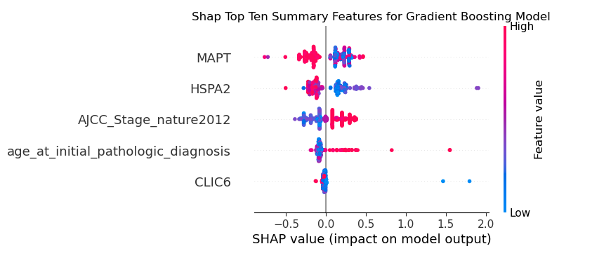
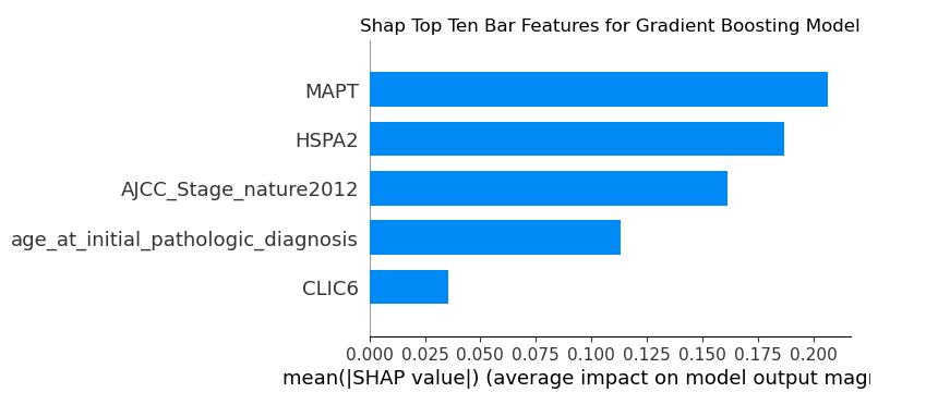
Gradient Boosting Model Features
For the Gradient Boosting model, two genes had the highest impact, followed by cancer stage at time of diagnosis
Logistic Regression Model Features
For the Logistic Regression model, Age_at_initial_pathologic_diagnosis had the biggest impact, followed by the HSPA2 gene and cancer stage at time of diagnosis.


Conclusions
The Cox PH and Gradient Boosting algorithms had the best survival prediction accuracy with respect to the “good” C-Index benchmark of 0.7. Cox PH beat out Gradient Boosting by a C-Index score of 0.734 to 0.721.
Looking across the three most accurate models, the features that had the biggest impact on predictions were:
- Age_at_initial_pathologic_diagnosis: Patient age at time of diagnosis
- AJCC_Stage_nature2012: Cancer stage at time of diagnosis
- HSPA2: Heat shock protein family A (Hsp70) member 2
- ELOVL2: ELOVL fatty acid elongase 2
- MAPT: Microtubule associated protein tau
Future work
- Run the analysis on the gene expression data only (exclude clinical data) to identify which genes are most predictive of overall survival
- Clustering analysis of samples
- Hyperparameter tuning. We could squeeze more accuracy out of these models with some hyperparameter tuning.
- Make the feature selection stage of the pipeline more specialized for each model
- Mitigate the imbalance in the data
- See how some of the deep learning survival algorithms perform on this data set
- See how well the model generalizes by testing it on some other breast cancer data sets
References
Footnotes
- ]Breast Cancer Statistics | How Common Is Breast Cancer? | American Cancer Society ↩︎
- TCGA Breast Cancer (BRCA) cohort data, Xena ↩︎
- Kwan-Moon Leung, Robert M. Elashoff, and Abdelmonem A., CENSORING ISSUES IN SURVIVAL ANALYSIS, Annual Review of Public Health
Vol. 18:83-104 (Volume publication date May 1997)
https://doi.org/10.1146/annurev.publhealth.18.1.83 ↩︎ - Martin Madera, Cancer Staging, https://www.healthit.gov/isa/taxonomy/term/2016/level-0 ↩︎
- Andrea Bommert, Thomas Welchowski, Matthias Schmid, Jörg Rahnenführer, Benchmark of filter methods for feature selection in high-dimensional gene expression survival data, Briefings in Bioinformatics, Volume 23, Issue 1, January 2022, bbab354, https://doi.org/10.1093/bib/bbab354 ↩︎
- Stack Overflow, How to calculate correlation between all columns and remove highly correlated ones using pandas? https://stackoverflow.com/questions/29294983/how-to-calculate-correlation-between-all-columns-and-remove-highly-correlated-on ↩︎
- Stefan Büttner, Boris Galjart, Berend R. Beumer et al, Quality and performance of validated prognostic models for survival after resection of intrahepatic cholangiocarcinoma: a systematic review and meta-analysis, HPB Online https://doi.org/10.1016/j.hpb.2020.07.007 ↩︎

2 thoughts on “Breast Cancer Survival Prediction: Algorithms and Survival Factors”