A falsification test for EV charging archetypes, run on 15,924 stations — and the one group of 838 that survived it
Almost every model of how electric vehicles will load the grid contains the same assumption, and it is usually stated so casually that it reads as description rather than as a modelling choice: that drivers fall into a small number of charging types.
The forecast S&P Global Commodity Insights prepared for PJM Interconnection is a clean example, because it writes the types down. On page 32 it defines five charging strategies, each in a phrase: “Starts to charge as soon as gets home, regardless of cost.” “Starts to charge as soon as on-peak pricing ends.” “Charges during super off-peak hours.” “Relies on public and workplace charging, starts to charge as soon as arrives to work.” “Typically relies on public charging.” Page 31 gives the mix and its trajectory: 94% Immediate / 6% Delayed in 2026, moving to 65% / 35% by 2046.
That mix is one of the most load-bearing numbers in the forecast. A twenty-year shift in the share of drivers who delay charging moves the evening peak, which moves the capacity requirement, which moves billions of dollars of investment. So it is worth asking a plain question about it: by what observation would you know the mix was wrong?
The question only has an answer if the categories it is defined over can be detected in data. I tested whether they can. The short version is that they mostly cannot — and that there is exactly one exception, which is the more interesting half of this piece.
The problem with the usual validation
The standard way to establish charging archetypes is to cluster session data and report an internal validity index — the elbow, a silhouette score, Davies–Bouldin, or a bootstrap stability measure. The literature is full of this. A 2026 study of 32,057 Korean stations reports six archetypes selected by elbow, silhouette and Davies–Bouldin, then validates them further by training four supervised classifiers to predict the cluster labels and reporting F1 above 0.994. A NeurIPS workshop paper from late 2025 identifies twelve archetypes across 8,000 US fast-charging sites, selecting k by forecasting loss.
None of these tests can distinguish a real group structure from no group structure at all. That is not a criticism of the authors; it is a property of the statistics. Christian Hennig made the point directly in 2007: “Stability is not the only aspect of cluster validity, and therefore a stable cluster is not guaranteed to be a meaningful pattern,” and “inflexible methods can yield meaningless but stable clusters.” Training a classifier on labels a clustering produced is worse still — it will recover them just as cleanly on a structureless cloud, because the labels are a deterministic function of the features.
k-means will always return k clusters. The question is never whether it returns them. It is whether it would have returned something different had the groups not been there.
The design
I used the EV WATTS public database — 13,937,235 charging sessions collected between 2019 and 2022, released to the public domain by the US Department of Energy. After cleaning, the population was 15,924 stations and 11,508,785 sessions: every station matched to site metadata with at least 200 sessions, across all venue types.
Each station is represented by 48 numbers: its distribution of session arrival hours, 24 for weekdays and 24 for weekends, jointly normalised and square-root transformed. Selection is by cluster stability — the median adjusted Rand index across all 4,950 pairs of 100 bootstrap replicates, at each k from 2 to 12.
The design’s whole content is what the observed curve is compared against. Three reference worlds, each resampled through the identical pipeline:
Reference A — one population. Every station drawn from a single shape plus its own sampling noise. This is the null most papers implicitly assume, and it is too weak to carry any conclusion.
Reference B — a continuum. A covariance-matched unimodal cloud, plus each station’s own noise. Stations differ from each other exactly as much as the real ones do, and along the same correlated directions — but by construction there are no groups in it. This is the reference that does the work, and it is the one nobody in the EV literature runs. The nearest published relative is Helgeson and Bair’s 2016 unimodal-null cluster significance test, from biostatistics.
Reference C — four real archetypes. A synthetic world containing exactly four discrete archetypes, at the same sample size and the same noise level. This is a positive control, and it is why the result below is a finding rather than a shrug. A null result with no demonstrated power is not evidence of anything.
The separation rule was fixed before the run: a curve separates from a reference only where its median exceeds that reference’s 97.5th percentile at the same k.
What happened
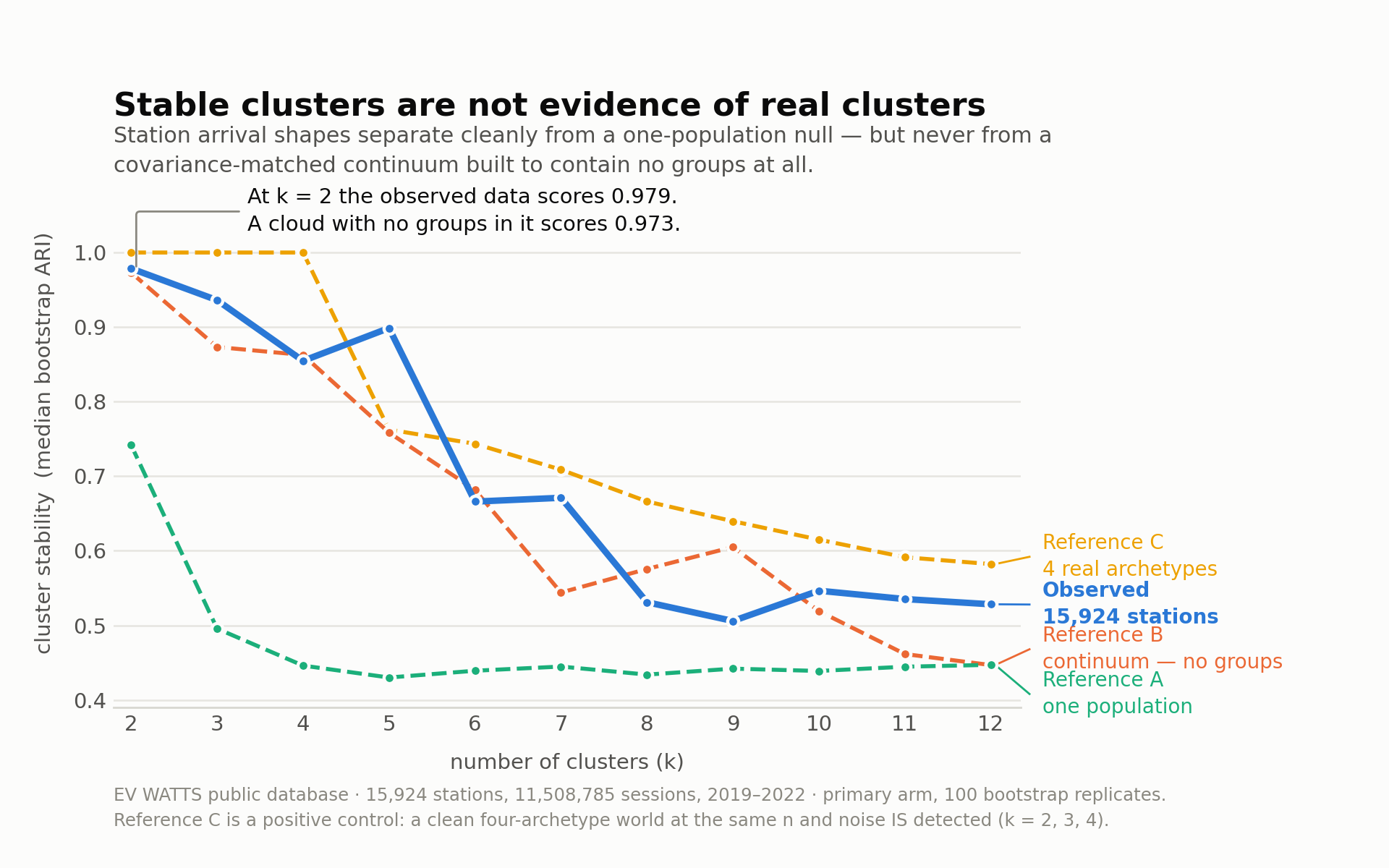
The observed data separates from Reference A at k = 2 through 7, with a best margin of +0.301. Stations genuinely do differ from one another by far more than sampling noise. Against the null most of the field uses, this looks like a resounding positive.
The observed data does not separate from Reference B at any k. The best margin is −0.013.
Reference C separates from Reference B at k = 2, 3 and 4. A clean four-archetype world at this sample size and this noise level is detected by the same protocol that failed to detect one in the real data.
And the number the whole exercise turns on: at k = 2, the observed stations score 0.979. The cloud with no groups in it scores 0.973. Anyone who clusters these shapes, reports “ARI ≈ 0.98 at k = 2, therefore two charging archetypes,” and stops there has reported an artifact of the algorithm. I know, because that is what my own first pass looked like before Reference B existed.
Three further checks:
- Holdout. 3,185 stations that never entered a fit reproduce the curve — 0.975 at k = 2, 0.847 at k = 4, 0.512 at k = 8. The shape of the curve is not an artifact of in-sample fitting.
- Robustness. Six arms — session thresholds of 100, 200 and 500, public venues only, per-block normalisation, and raw shares without the square root. Four isolated separations from Reference B appeared across all of them. The rule was applied 66 times at a 97.5th percentile, where 1.65 separations are expected by chance. None was in the primary arm, no two arms agreed on a k, and three of the four had margins under 0.03. That is what chance looks like.
- Reference calibration. Reference B’s realised feature variance against the observed data is 0.990–1.006 across five of the six arms (primary 1.006, threshold 100 1.004, threshold 500 0.990, public-only 1.004, per-block 1.005). The sixth, raw shares, comes in at 0.874, because clipping bites harder without the square root. An under-dispersed reference makes separation artificially easier, so that arm’s negative result is conservative rather than compromised.
A continuum is not the absence of structure
This gets misread, so it is worth being blunt: the finding is the absence of discrete types, not the absence of structure. Structure is abundant.
Cluster membership is strongly associated with venue — Cramér’s V of 0.685 at k = 2 and 0.492 at k = 4 — and with the number of ports at the station (0.42). It is weakly associated with census region (0.16–0.18) and barely at all with land use (0.06). Where a charger is sited predicts its shape well. What it does not do is sort stations into kinds.
At k = 4 the partition is perfectly legible: a workplace-heavy group peaking at 08:00, a flat all-day group, an evening-peaking residential group, and a small, sharp late-night one. It is tempting to read those four as the archetypes recovered. Mostly they are not. They are regions of a smooth cloud, and the same fit run on Reference B produces four equally legible groups from data guaranteed to contain none.
Mostly.
The exception
There was one thing in that k = 4 fit I could not explain away. Three of the four clusters were ordinary regions of a continuum. The fourth — 838 stations, about 5% of the population — was not behaving like the others.
A global stability curve cannot answer that question. It scores the whole partition at once, so it is dominated by the three clusters that dissolve; a small, well-separated group can hide inside an unstable partition of everything else and never show up. So I ran a second, narrower test: cluster-wise bootstrap Jaccard for that one group, against each reference world’s own best cluster of four, with the rule fixed in advance exactly as before.
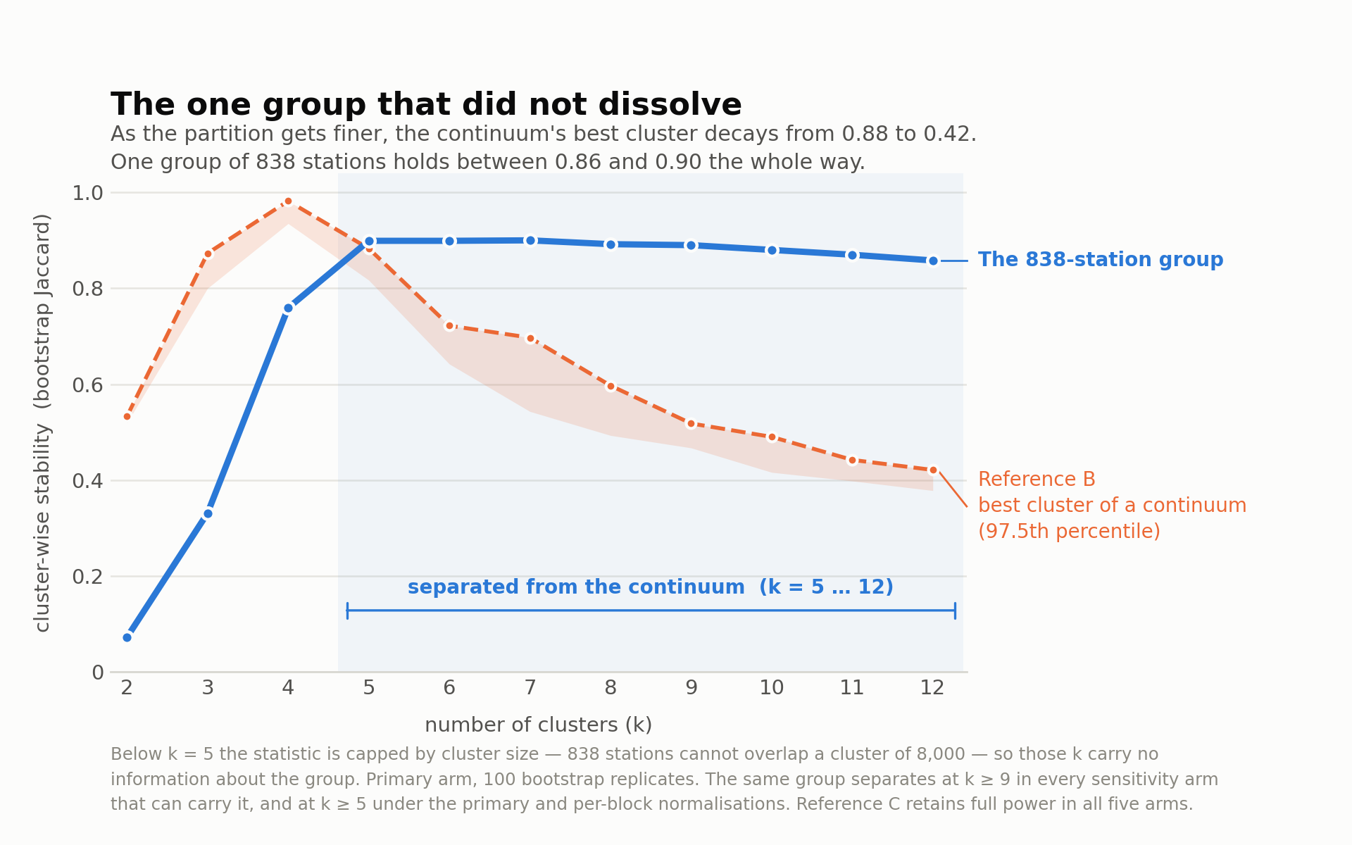
As the partition gets finer, the continuum’s best cluster decays from 0.88 to 0.42 — that is what a region of a smooth cloud does when you cut it more ways. The 838-station group holds between 0.858 and 0.900 the whole way, and separates from the continuum at k = 5 through 12: eight of eleven comparisons, contiguous, where 0.275 are expected by chance, with margins growing from +0.016 to +0.437. Reference C separates at all eleven k, so the statistic has full power here.
Two details make this more than a curve crossing. Leakage collapses to 0.006 — once the partition is fine enough to hold the group, its members are essentially never assigned alongside non-members. The group stays together and stays apart, which is the half a Jaccard alone would not show. And Reference B’s own k = 4 partition is four roughly equal clusters, 2,664 to 5,124 stations, with no small one. A covariance-matched continuum does not produce a small tight cluster when asked for four. The data does.
The group does not separate at k = 2, 3 or 4, and that is arithmetic rather than evidence: Jaccard is bounded above by a size ratio, so 838 stations cannot overlap a cluster of 8,000. Those k carry no information about the group. k = 4 would have been the least informative hit in any case — the group is defined there, so recovering it would be the definition reproducing itself.
What survives stress-testing, and what narrows
I had originally waived the sensitivity arms on the argument that they exist to stress a global finding. That argument does not survive a positive result, so I ran them.
| arm | of the 838 kept | separated from the continuum at |
|---|---|---|
| primary | 100% | k = 5 … 12 |
| per-block normalisation | 100% | k = 5 … 12 |
| 500-session threshold | 28% | k = 6 … 12 |
| 100-session threshold | 100% | k = 9 … 12 |
| raw shares, no square root | 100% | k = 9 … 12 |
| public venues only | 0.5% | not runnable |
No arm produced a negative, and Reference C kept full power in all five runnable arms — so nothing here is the statistic running out of steam. Across 55 comparisons where 1.375 are expected by chance, 31 separations were observed, in four contiguous runs. But two arms genuinely narrow the range, so the honest statement of the finding names the range rather than the primary arm’s: the group separates from a continuum at k ≥ 9 under every configuration that can carry it, and from k ≥ 5 under the primary and per-block normalisations.
Three things in that table are worth more than the pass/fail.
Lowering the threshold does not dissolve the group — it grows it. Admitting stations with 100–199 sessions adds 6,124 units, and the group’s score drops to 0.589–0.608. That looks like decay until you count. In the arm’s own fit, 833 of the 838 still land in a single cluster — but the cluster now holds 1,810 stations, 38% of them newly admitted. At k = 12, only 135 of the 838 have left; a cluster containing exactly the 703 that stay would score 0.839, near the primary arm’s 0.858. The drop is a denominator effect. More stations share this shape than the 200-session threshold was showing me.
The public-venues arm is not a failure, it is a disclosure. Four of the 838 stations survive it. The group is 99.2% single-family residential, and the public-venue scope contains no residential class at all, so the arm does not stress this finding — it deletes the population the finding is about. That tells you something I should state plainly: this is a residential-charging result and always was.
And one arm fails a reference. At the 100-session threshold the group does not separate from Reference A — the weak null — at any k. The reason is instructive: Reference A’s best cluster at that arm is a single blob of 11,932 stations, 54% of the population, the same one at every k. A majority cluster in a structureless world is reproducible because there is nothing to cut it differently, not because it is a group. That is a defect of Reference A as a comparator, not evidence about the data, and I am reporting it because the arm is otherwise reported as passing.
The hour is real. The reason is not established.
The group’s arrivals concentrate in a single hour: 48.3% of them fall at 23:00 (45.2% of the weekday distribution alone), against 0.028 in the 22:00 bin and 0.030 in the 00:00 bin. It is 99.2% single-family residential, 99.8% Level 2, 99.5% free to use, 99.4% single-port, and it is 13% of all single-family residential stations in the data — a slice of that population, not the whole of it.
A spike that sharp in a late hour is exactly what a daylight-saving handling bug would manufacture, so that had to be ruled out before the hour could be named. I ran a per-station DST screen against the real spring and autumn transitions, with placebo windows as a control. The estimated offset is −0.005, with a 95% interval of [−0.0075, +0.0025]; the 23:00 share is 0.643 before and 0.658 after the spring transition and does not move; 3 of 385 testable stations detect, against a 5% null. The same estimator applied to Phoenix — which does not observe DST — returns +0.555, so the test has power. 23:00 is 23:00.
Which brings me to the part I cannot resolve, and which I think is the most useful thing in this piece.
The obvious reading is a time-of-use tariff: drivers on a rate whose off-peak window opens at 23:00. I am not going to make that claim, because a second explanation fits the evidence at least as well. The dataset contains no rate schedule, no tariff identifier, and no charging-network, vendor or provider field of any kind. So the group could equally be one vendor’s, one utility programme’s, or one pilot’s residential units, shipped with a scheduled start time — which would produce a 48% single-hour concentration with no driver behaviour in it at all.
I lean toward the second, and the reason is that a 48% single-hour spike is more precise than human price response usually is. The group’s geography points the same way: it is 46.5% East North Central, and 26.5% of it sits in a single metro area, where it accounts for 26.5% of that metro’s stations against 5.3% across the population.
The distinction matters more than it might appear. If it is a tariff response, it is a measurement of demand response and it is worth a great deal to anyone designing an EV rate. If it is a shipped default, it is a measurement of a procurement decision — real, useful for load forecasting, and almost worthless as evidence about how drivers behave. Separating the two requires a source this dataset does not contain, and it is the next thing I intend to chase.
What this does not say
It does not show that the five assumed strategies are false. They are driver-level descriptions of home-charging behaviour. I clustered stations. Those are different units, and no test on one directly refutes a claim about the other. What the result does show is that the taxonomy is not recoverable from the largest public observational dataset of US charging that exists — which makes it an unvalidated modelling convenience rather than an empirical regularity, and makes the 94/6-to-65/35 trajectory a parameter with no observational check attached.
This is a claim about arrivals, not about load. The features are the hours sessions start. An arrival distribution is not a load shape, and I have been careful not to let the two words trade places.
The dataset contains zero Tesla or NACS connectors. The strongest counter-hypothesis to everything above is that the archetypes exist and live in the network this data does not see. That bites hardest on the 838-station group, which is residential Level 2 charging in a dataset with no Tesla home charging in it.
The group is a shape, not a count. There is no sampling frame here, so “about 5%” is 5% of this dataset’s matched stations at this threshold and of nothing else. It cannot be scaled to the US residential fleet, and no absolute megawatt or household figure follows from it.
Its boundary is soft. 695 of the 838 survive at the finest partition; the rest are a fringe that fine cuts peel away. Any downstream use should treat membership as a matter of degree.
Shapes are pooled across 2019–2022, over which I have separately measured a median total-variation distance of 0.038 to 0.068 between consecutive period pairs. Pooling across a drifting population could smear genuinely separated types into an apparent continuum, and it cuts sharper for the group than for the global result — a tariff or a programme has a start date. This is the strongest technical objection available, and it is not corrected for.
Reference C is an upper bound on detectability. It has no within-archetype variation, so the power statement reads “a clean four-archetype world would have been detected,” not “any archetype structure would.”
What I would take from this
The modelling instruction is narrow and, I think, usable: condition on venue and time, which are observable and predictive. Do not condition on behavioural type, which is neither — unless you can show the type separates from a continuum, in which case say which k range it holds across.
That is roughly where the industry’s own guidance already points. ESIG’s EV Load Forecasting Guide, published March 2026, frames charging behaviour by siting use case — “Where the EVSE has been sited determines the type of vehicles that will charge at the station” — rather than by driver archetype, and its Best Practice 14 asks forecasters to “calibrate charging profiles by benchmarking against real-world metered data.” ISO New England’s 2026 EV forecast does the same thing structurally: “Charging profiles define the hourly allocation of daily charging energy,” by month and day type, with no archetype mix in it at all.
Reproducing it
The stability protocol and all three reference generators are public and Apache-2.0, at github.com/jaksanders/evbench-null. That package is the reusable part: it knows nothing about EV charging, it takes any count matrix, and it ships the twenty control tests — a positive control with real archetypes and a negative control with none — that are the only reason to believe a number it emits. Its cluster.py is byte-identical to the file that produced the results above, and the README gives its SHA-256 so that can be checked when the rest opens.
The cleaning pipeline carries the same licence but is not public yet; it is a deliverable in its own right and is released with the shape library. The run emits a run identifier that hashes the git SHA, the configuration and the SHA-256 of every input, so a third party can confirm they ran the same thing I did — which is a claim I would rather have checked than believed, and one I cannot fully make good on until that release. As an external check on the cleaning, the same pipeline reproduces NREL’s published EV WATTS utilization figures to within 2%, with a correlation of 0.975.
No published artifact contains a station identifier. The group is 838 stations at 99.2% single-family residential, which is the worst case for re-identification, so per-station statistics stay unpublished.
If you cluster charging data, the reference generators are the part worth taking. Five questions are worth asking of any archetype claim, including mine:
- What null were the clusters compared against?
- Was the reference variance-matched to the observed data, and what was the realised ratio?
- Would the method have detected k archetypes if they existed — where is the positive control?
- How many times was the selection rule applied, and how many separations are expected by chance?
- Do the clusters reproduce on held-out units, and across the choices you could have made differently?
I am not aware of any published work that applies a null-reference test to EV charging behaviour. That is a search result rather than a census, and I would be glad to be corrected.
Sources
- S&P Global Commodity Insights, Electric Vehicle Charging Power Demand Forecast — PJM Interconnection, 19 September 2025; posted as PJM Load Analysis Subcommittee reference material, 28 October 2025. Strategies p.32, mix p.31. https://www.pjm.com/-/media/DotCom/committees-groups/subcommittees/las/2025/20251028/20251028-reference—spglobal—pjm-ev-forecast.pdf
- ISO New England, Final 2026 Electric Vehicle Forecast, 1 May 2026, pp.19–20. https://www.iso-ne.com/static-assets/documents/100034/transfx2026final.pdf
- ESIG, EV Load Forecasting Guide, March 2026 (Giraldez, Morash, Steffen, Mandelman). https://www.esig.energy/reports-briefs/ev-load-forecasting/
- EV WATTS Public Database, US DOE. https://www.osti.gov/biblio/1970735
- J. Sanders, evbench-null: null-reference testing for load-shape clustering, 2026. Apache-2.0. https://github.com/jaksanders/evbench-null
- NREL/CP-5400-85902, Evaluating Electric Vehicle Public Charging Utilization in the United States Using the EV WATTS Dataset. https://docs.nrel.gov/docs/fy24osti/85902.pdf
- C. Hennig, “Cluster-wise assessment of cluster stability”, Computational Statistics & Data Analysis, 2007.
- E. Helgeson and E. Bair, “Non-Parametric Cluster Significance Testing with Reference to a Unimodal Null Distribution”, 2016. https://arxiv.org/abs/1610.01424
- R. Tibshirani, G. Walther and T. Hastie, “Estimating the number of clusters in a data set via the gap statistic”, JRSS-B 63(2), 2001.
- S. Powell, G. V. Cezar, L. Min, I. Azevedo and R. Rajagopal, “Charging infrastructure access and operation to reduce the grid impacts of deep electric vehicle adoption”, Nature Energy 7, 2022. https://www.nature.com/articles/s41560-022-01105-7
- K. Nikhal, B. S. Riggan, L. Ackerknecht and P. Stahlfeld, “Discovering EV Charging Site Archetypes Through Few-Shot Forecasting”, NeurIPS 2025 Workshop on Tackling Climate Change with ML. https://arxiv.org/abs/2510.26910
- Ü. Yılmaz, “Behavioral Clustering and Load Characterization of EV Charging Stations”, Processes 14(11):1692, 2026. https://doi.org/10.3390/pr14111692
 James Sanders